Aula10

Três ou mais tratamentos

Anova 1 fator

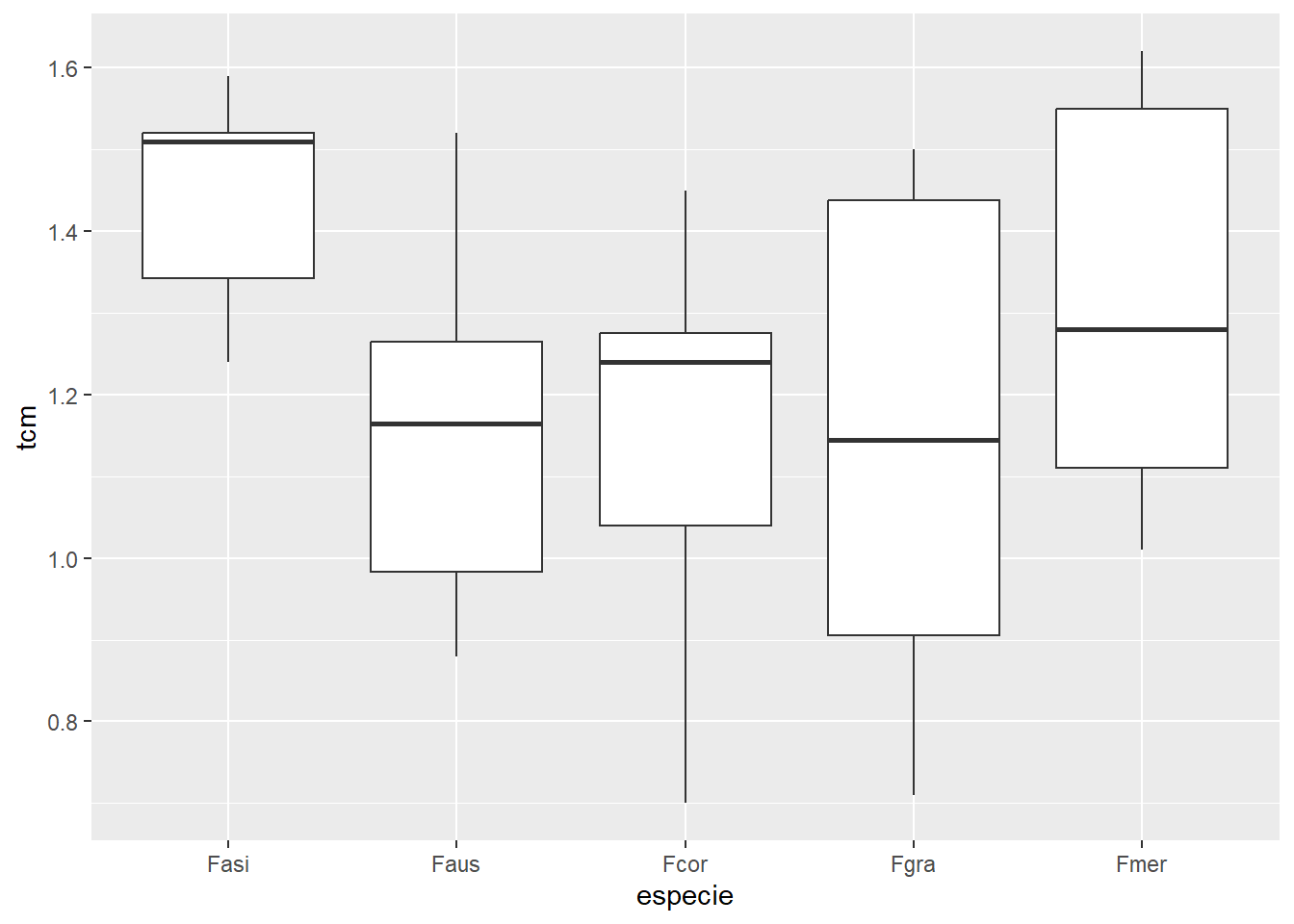
Experimento com um fator e em delineamento inteiramente casualizado para comparar o crescimento micelial de diferentes espécies de um fungo fitopatogênico. A resposta a ser estudada é a TCM = taxa de crescimento micelial.

Preparo

library(readxl)
library(tidyverse)

Warning: package 'ggplot2' was built under R version 4.2.3

Warning: package 'tibble' was built under R version 4.2.3

Warning: package 'dplyr' was built under R version 4.2.3

── Attaching core tidyverse packages ──────────────────────── tidyverse 2.0.0 ──
✔ dplyr     1.1.2     ✔ readr     2.1.4
✔ forcats   1.0.0     ✔ stringr   1.5.0
✔ ggplot2   3.4.2     ✔ tibble    3.2.1
✔ lubridate 1.9.2     ✔ tidyr     1.3.0
✔ purrr     1.0.1     
── Conflicts ────────────────────────────────────────── tidyverse_conflicts() ──
✖ dplyr::filter() masks stats::filter()
✖ dplyr::lag()    masks stats::lag()
ℹ Use the conflicted package (<http://conflicted.r-lib.org/>) to force all conflicts to become errors

micelial <- read_excel("dados-diversos.xlsx", "micelial")
head(micelial)

# A tibble: 6 × 3
  especie   rep   tcm
  <chr>   <dbl> <dbl>
1 Fasi        1  1.5 
2 Fasi        2  1.59
3 Fasi        3  1.52
4 Fasi        4  1.52
5 Fasi        5  1.24
6 Fasi        6  1.29

micelial %>%
  ggplot(aes(especie, tcm)) +
  geom_boxplot()

Premissas

Modelo usando aov()

aov1 <- aov(tcm ~ especie, 
            data = micelial)
summary(aov1)

            Df Sum Sq Mean Sq F value Pr(>F)
especie      4 0.4692 0.11729   1.983  0.117
Residuals   37 2.1885 0.05915               

library(performance)

Warning: package 'performance' was built under R version 4.2.3

check_heteroscedasticity(aov1)

OK: Error variance appears to be homoscedastic (p = 0.175).

check_normality(aov1)

OK: residuals appear as normally distributed (p = 0.074).

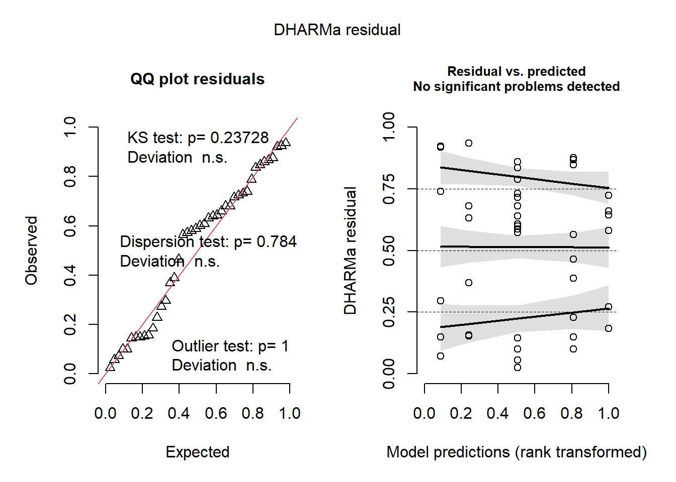
library(DHARMa)

This is DHARMa 0.4.6. For overview type '?DHARMa'. For recent changes, type news(package = 'DHARMa')

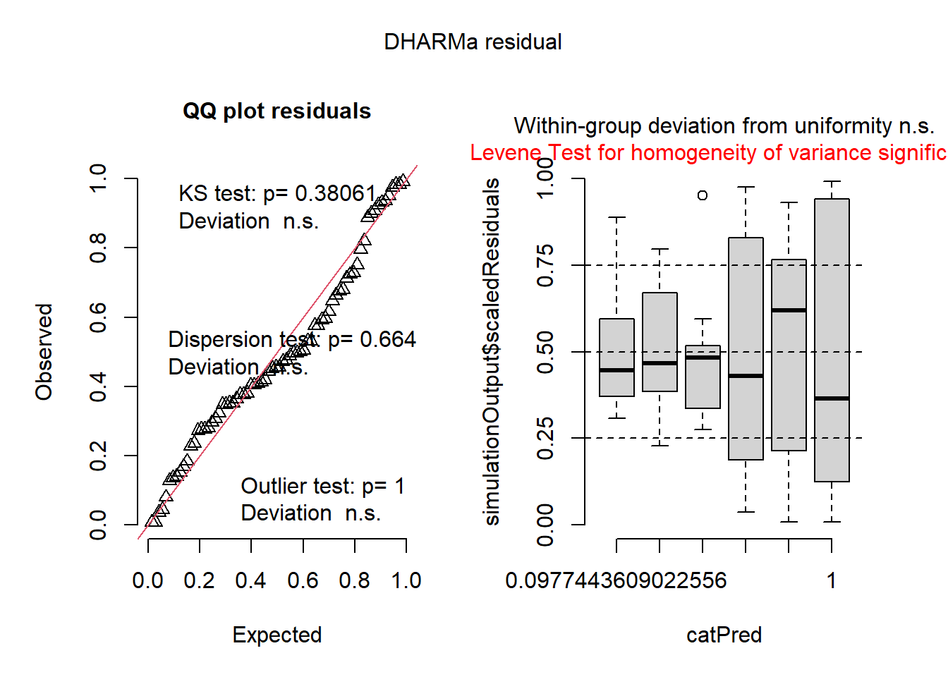
plot(simulateResiduals(aov1))

Warning in checkModel(fittedModel): DHARMa: fittedModel not in class of
supported models. Absolutely no guarantee that this will work!

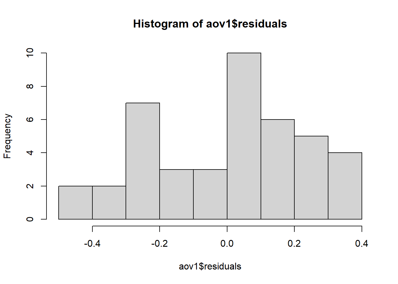
# teste de normalidade
hist(aov1$residuals)

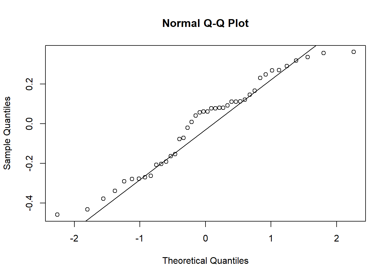
qqnorm(aov1$residuals)
qqline(aov1$residuals)

shapiro.test(aov1$residuals)

    Shapiro-Wilk normality test

data:  aov1$residuals
W = 0.95101, p-value = 0.07022

Interpretação

Premissas da anova atendidas. Efeito não significativo de espécies.

E quanto não atende às premissas?

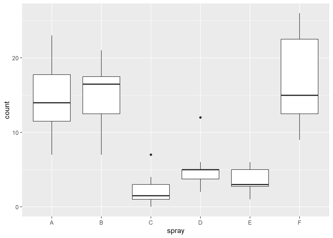
Efeito de inseticida na mortalidade de insetos (Beall, 1942). The Transformation of data from entomological field experiments, Biometrika, 29, 243–262. Dados no pacote “datasets” do R. data(InsectSprays)

insects <- tbl_df(InsectSprays) |> 
  select(spray, count)

Warning: `tbl_df()` was deprecated in dplyr 1.0.0.
ℹ Please use `tibble::as_tibble()` instead.

insects %>%
  ggplot(aes(spray, count))+
  geom_boxplot() 

Anova paramétrica

aov2 <- aov(count ~ spray, data = insects)
summary(aov2)

            Df Sum Sq Mean Sq F value Pr(>F)    
spray        5   2669   533.8    34.7 <2e-16 ***
Residuals   66   1015    15.4                   
---
Signif. codes:  0 '***' 0.001 '**' 0.01 '*' 0.05 '.' 0.1 ' ' 1

check_normality(aov2)

Warning: Non-normality of residuals detected (p = 0.022).

check_heteroscedasticity(aov2)

Warning: Heteroscedasticity (non-constant error variance) detected (p < .001).

plot(simulateResiduals(aov2))

Warning in checkModel(fittedModel): DHARMa: fittedModel not in class of
supported models. Absolutely no guarantee that this will work!

library(emmeans)

Warning: package 'emmeans' was built under R version 4.2.3

aov2_means <- emmeans(aov2, ~ spray,
                      type = "response")
aov2_means

 spray emmean   SE df lower.CL upper.CL
 A      14.50 1.13 66   12.240    16.76
 B      15.33 1.13 66   13.073    17.59
 C       2.08 1.13 66   -0.177     4.34
 D       4.92 1.13 66    2.656     7.18
 E       3.50 1.13 66    1.240     5.76
 F      16.67 1.13 66   14.406    18.93

Confidence level used: 0.95 

pwpm(aov2_means)

        A       B       C       D       E       F
A [14.50]  0.9952  <.0001  <.0001  <.0001  0.7542
B  -0.833 [15.33]  <.0001  <.0001  <.0001  0.9603
C  12.417  13.250 [ 2.08]  0.4921  0.9489  <.0001
D   9.583  10.417  -2.833 [ 4.92]  0.9489  <.0001
E  11.000  11.833  -1.417   1.417 [ 3.50]  <.0001
F  -2.167  -1.333 -14.583 -11.750 -13.167 [16.67]

Row and column labels: spray
Upper triangle: P values   adjust = "tukey"
Diagonal: [Estimates] (emmean)   type = "response"
Lower triangle: Comparisons (estimate)   earlier vs. later

library(multcomp)

Carregando pacotes exigidos: mvtnorm

Carregando pacotes exigidos: survival

Warning: package 'survival' was built under R version 4.2.3

Carregando pacotes exigidos: TH.data

Warning: package 'TH.data' was built under R version 4.2.3

Carregando pacotes exigidos: MASS

Warning: package 'MASS' was built under R version 4.2.3

Attaching package: 'MASS'

The following object is masked from 'package:dplyr':

    select

Attaching package: 'TH.data'

The following object is masked from 'package:MASS':

    geyser

library(multcompView)

Warning: package 'multcompView' was built under R version 4.2.3

cld(aov2_means)

 spray emmean   SE df lower.CL upper.CL .group
 C       2.08 1.13 66   -0.177     4.34  1    
 E       3.50 1.13 66    1.240     5.76  1    
 D       4.92 1.13 66    2.656     7.18  1    
 A      14.50 1.13 66   12.240    16.76   2   
 B      15.33 1.13 66   13.073    17.59   2   
 F      16.67 1.13 66   14.406    18.93   2   

Confidence level used: 0.95 
P value adjustment: tukey method for comparing a family of 6 estimates 
significance level used: alpha = 0.05 
NOTE: If two or more means share the same grouping symbol,
      then we cannot show them to be different.
      But we also did not show them to be the same. 

Qualidade ajuste do modelo

# não paramétrico
kruskal.test(count ~ spray, data = insects)

    Kruskal-Wallis rank sum test

data:  count by spray
Kruskal-Wallis chi-squared = 54.691, df = 5, p-value = 1.511e-10

library(agricolae)
kruskal(insects$count, insects$spray, 
        console = TRUE)

Study: insects$count ~ insects$spray
Kruskal-Wallis test's
Ties or no Ties

Critical Value: 54.69134
Degrees of freedom: 5
Pvalue Chisq  : 1.510845e-10 

insects$spray,  means of the ranks

  insects.count  r
A      52.16667 12
B      54.83333 12
C      11.45833 12
D      25.58333 12
E      19.33333 12
F      55.62500 12

Post Hoc Analysis

t-Student: 1.996564
Alpha    : 0.05
Minimum Significant Difference: 8.462804 

Treatments with the same letter are not significantly different.

  insects$count groups
F      55.62500      a
B      54.83333      a
A      52.16667      a
D      25.58333      b
E      19.33333     bc
C      11.45833      c

Modelo linear generalizado

glm1 <- glm(count ~ spray,
  data = insects,
  family = poisson(link = "identity"))
plot(simulateResiduals(glm1))

summary(glm1)

Call:
glm(formula = count ~ spray, family = poisson(link = "identity"), 
    data = insects)

Deviance Residuals: 
    Min       1Q   Median       3Q      Max  
-2.3852  -0.8876  -0.1482   0.6063   2.6922  

Coefficients:
            Estimate Std. Error z value Pr(>|z|)    
(Intercept)  14.5000     1.0992  13.191  < 2e-16 ***
sprayB        0.8333     1.5767   0.529    0.597    
sprayC      -12.4167     1.1756 -10.562  < 2e-16 ***
sprayD       -9.5833     1.2720  -7.534 4.92e-14 ***
sprayE      -11.0000     1.2247  -8.981  < 2e-16 ***
sprayF        2.1667     1.6116   1.344    0.179    
---
Signif. codes:  0 '***' 0.001 '**' 0.01 '*' 0.05 '.' 0.1 ' ' 1

(Dispersion parameter for poisson family taken to be 1)

    Null deviance: 409.041  on 71  degrees of freedom
Residual deviance:  98.329  on 66  degrees of freedom
AIC: 376.59

Number of Fisher Scoring iterations: 3

glm1_means <- emmeans(glm1, ~ spray)
cld(glm1_means)

 spray emmean    SE  df asymp.LCL asymp.UCL .group
 C       2.08 0.417 Inf      1.27      2.90  1    
 E       3.50 0.540 Inf      2.44      4.56  12   
 D       4.92 0.640 Inf      3.66      6.17   2   
 A      14.50 1.099 Inf     12.35     16.65    3  
 B      15.33 1.130 Inf     13.12     17.55    3  
 F      16.67 1.179 Inf     14.36     18.98    3  

Confidence level used: 0.95 
P value adjustment: tukey method for comparing a family of 6 estimates 
significance level used: alpha = 0.05 
NOTE: If two or more means share the same grouping symbol,
      then we cannot show them to be different.
      But we also did not show them to be the same. 

Anova não paramétrica

insects

# A tibble: 72 × 2
   spray count
   <fct> <dbl>
 1 A        10
 2 A         7
 3 A        20
 4 A        14
 5 A        14
 6 A        12
 7 A        10
 8 A        23
 9 A        17
10 A        20
# ℹ 62 more rows

kruskal.test(count ~ spray, data = insects)

    Kruskal-Wallis rank sum test

data:  count by spray
Kruskal-Wallis chi-squared = 54.691, df = 5, p-value = 1.511e-10

library(agricolae)
attach(insects)
kruskal(insects$count, insects$spray, console = TRUE)

Study: insects$count ~ insects$spray
Kruskal-Wallis test's
Ties or no Ties

Critical Value: 54.69134
Degrees of freedom: 5
Pvalue Chisq  : 1.510845e-10 

insects$spray,  means of the ranks

  insects.count  r
A      52.16667 12
B      54.83333 12
C      11.45833 12
D      25.58333 12
E      19.33333 12
F      55.62500 12

Post Hoc Analysis

t-Student: 1.996564
Alpha    : 0.05
Minimum Significant Difference: 8.462804 

Treatments with the same letter are not significantly different.

  insects$count groups
F      55.62500      a
B      54.83333      a
A      52.16667      a
D      25.58333      b
E      19.33333     bc
C      11.45833      c

GLM família poisson

# distribuição da resposta
attach(insects)

The following objects are masked from insects (pos = 3):

    count, spray

insects

# A tibble: 72 × 2
   spray count
   <fct> <dbl>
 1 A        10
 2 A         7
 3 A        20
 4 A        14
 5 A        14
 6 A        12
 7 A        10
 8 A        23
 9 A        17
10 A        20
# ℹ 62 more rows

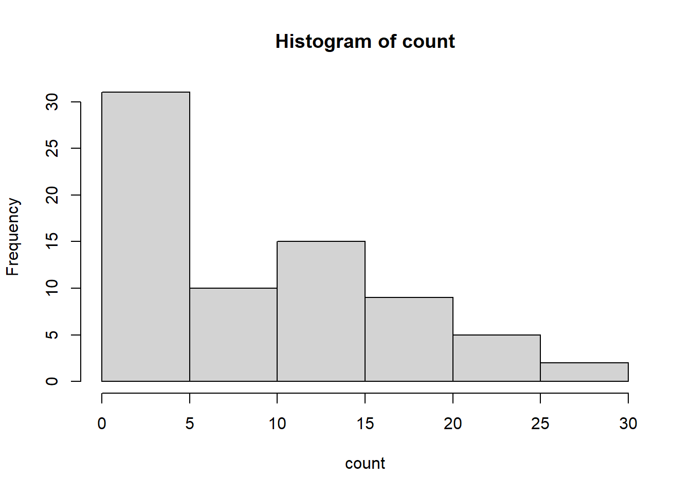
hist(count)

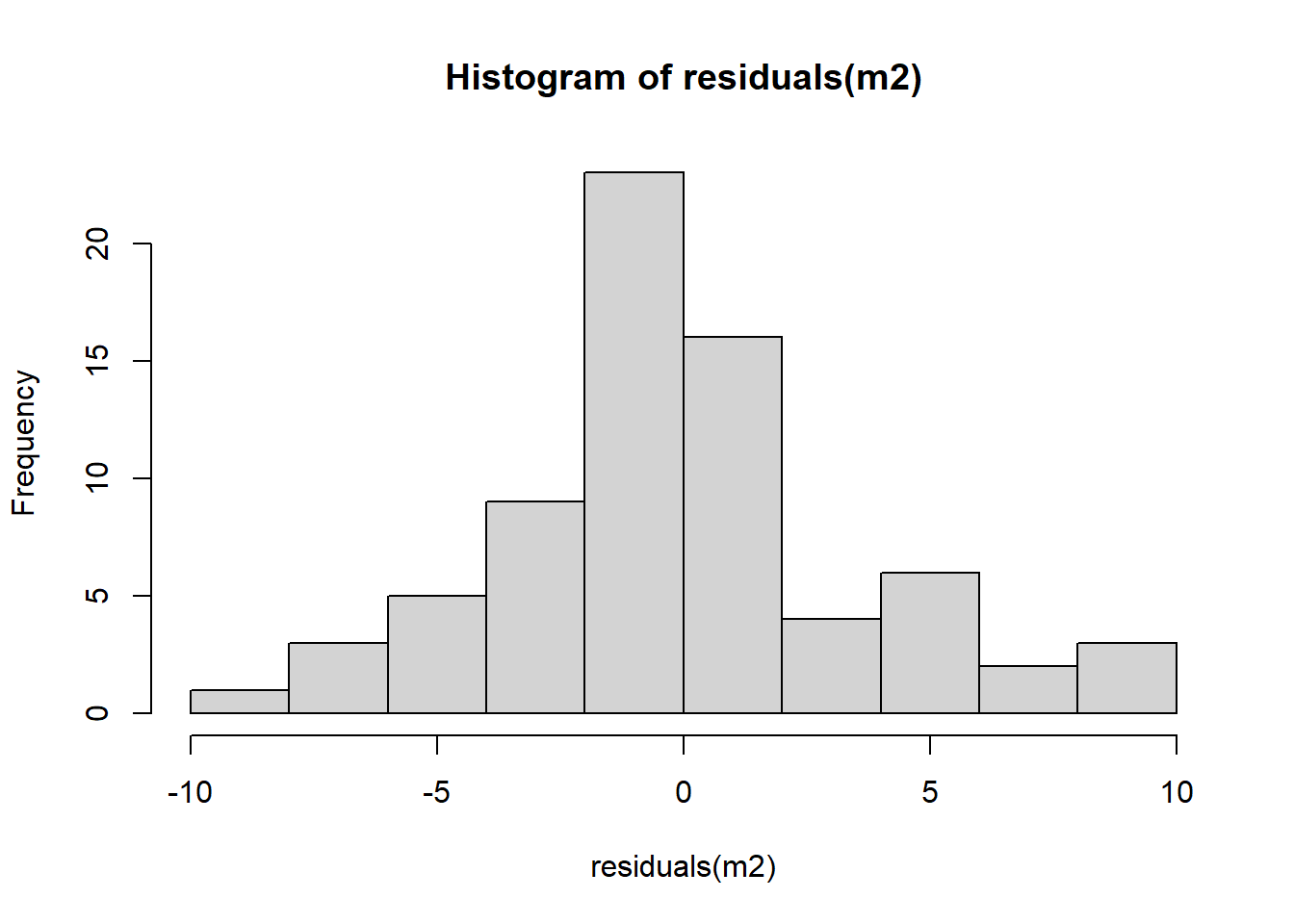
# modelo linear generalizado
m2 <- lm(count ~ spray, data = insects)
summary(m2)

Call:
lm(formula = count ~ spray, data = insects)

Residuals:
   Min     1Q Median     3Q    Max 
-8.333 -1.958 -0.500  1.667  9.333 

Coefficients:
            Estimate Std. Error t value Pr(>|t|)    
(Intercept)  14.5000     1.1322  12.807  < 2e-16 ***
sprayB        0.8333     1.6011   0.520    0.604    
sprayC      -12.4167     1.6011  -7.755 7.27e-11 ***
sprayD       -9.5833     1.6011  -5.985 9.82e-08 ***
sprayE      -11.0000     1.6011  -6.870 2.75e-09 ***
sprayF        2.1667     1.6011   1.353    0.181    
---
Signif. codes:  0 '***' 0.001 '**' 0.01 '*' 0.05 '.' 0.1 ' ' 1

Residual standard error: 3.922 on 66 degrees of freedom
Multiple R-squared:  0.7244,    Adjusted R-squared:  0.7036 
F-statistic:  34.7 on 5 and 66 DF,  p-value: < 2.2e-16

anova(m2)

Analysis of Variance Table

Response: count
          Df Sum Sq Mean Sq F value    Pr(>F)    
spray      5 2668.8  533.77  34.702 < 2.2e-16 ***
Residuals 66 1015.2   15.38                      
---
Signif. codes:  0 '***' 0.001 '**' 0.01 '*' 0.05 '.' 0.1 ' ' 1

m4 <- glm(count ~ spray,
  data = insects,
  family = poisson(link = "identity")
)

summary(m4)

Call:
glm(formula = count ~ spray, family = poisson(link = "identity"), 
    data = insects)

Deviance Residuals: 
    Min       1Q   Median       3Q      Max  
-2.3852  -0.8876  -0.1482   0.6063   2.6922  

Coefficients:
            Estimate Std. Error z value Pr(>|z|)    
(Intercept)  14.5000     1.0992  13.191  < 2e-16 ***
sprayB        0.8333     1.5767   0.529    0.597    
sprayC      -12.4167     1.1756 -10.562  < 2e-16 ***
sprayD       -9.5833     1.2720  -7.534 4.92e-14 ***
sprayE      -11.0000     1.2247  -8.981  < 2e-16 ***
sprayF        2.1667     1.6116   1.344    0.179    
---
Signif. codes:  0 '***' 0.001 '**' 0.01 '*' 0.05 '.' 0.1 ' ' 1

(Dispersion parameter for poisson family taken to be 1)

    Null deviance: 409.041  on 71  degrees of freedom
Residual deviance:  98.329  on 66  degrees of freedom
AIC: 376.59

Number of Fisher Scoring iterations: 3

anova(m4)

Analysis of Deviance Table

Model: poisson, link: identity

Response: count

Terms added sequentially (first to last)

      Df Deviance Resid. Df Resid. Dev
NULL                     71     409.04
spray  5   310.71        66      98.33

hist(residuals(m2))

hist(residuals(m4))

# resultados extraidos da lista
library(broom)
tidy(m4)

# A tibble: 6 × 5
  term        estimate std.error statistic  p.value
  <chr>          <dbl>     <dbl>     <dbl>    <dbl>
1 (Intercept)   14.5        1.10    13.2   9.90e-40
2 sprayB         0.833      1.58     0.529 5.97e- 1
3 sprayC       -12.4        1.18   -10.6   4.45e-26
4 sprayD        -9.58       1.27    -7.53  4.92e-14
5 sprayE       -11.0        1.22    -8.98  2.67e-19
6 sprayF         2.17       1.61     1.34  1.79e- 1

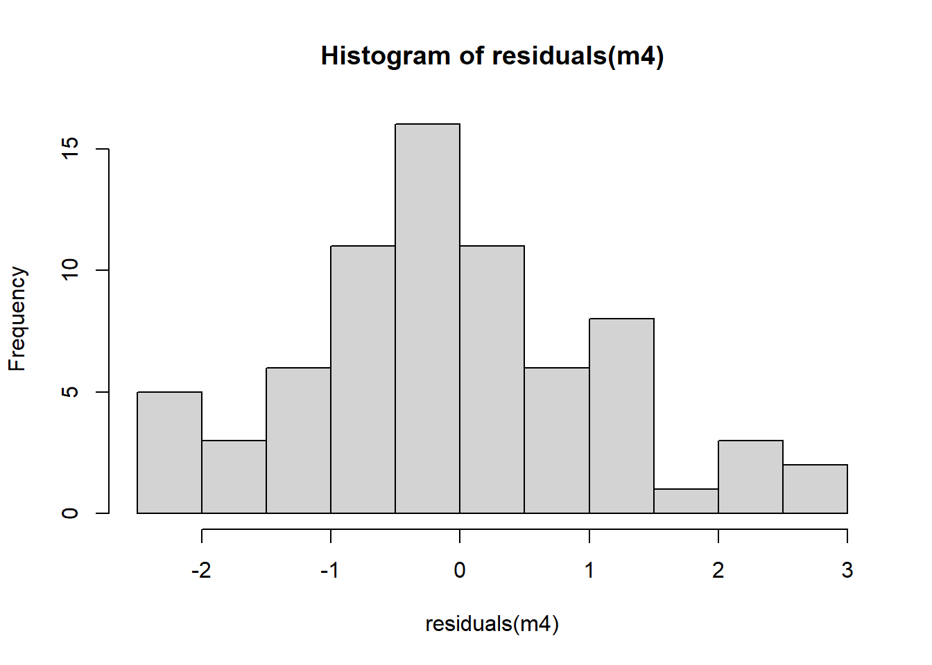
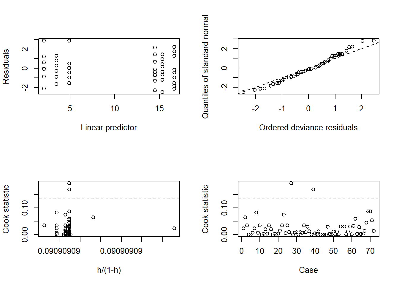
# ajuste do modelo
library(boot)
m4.diag <- glm.diag(m4)
glm.diag.plots(m4, glm.diag(m4))

Comparação de médias

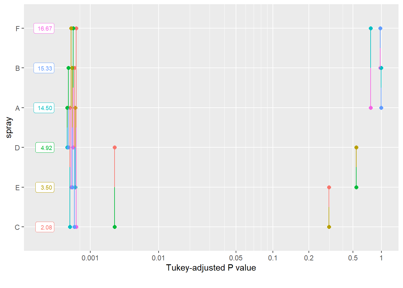
library(emmeans)
em <- emmeans(m4, ~spray)
pwpp(em)

multcomp::cld(em) 

 spray emmean    SE  df asymp.LCL asymp.UCL .group
 C       2.08 0.417 Inf      1.27      2.90  1    
 E       3.50 0.540 Inf      2.44      4.56  12   
 D       4.92 0.640 Inf      3.66      6.17   2   
 A      14.50 1.099 Inf     12.35     16.65    3  
 B      15.33 1.130 Inf     13.12     17.55    3  
 F      16.67 1.179 Inf     14.36     18.98    3  

Confidence level used: 0.95 
P value adjustment: tukey method for comparing a family of 6 estimates 
significance level used: alpha = 0.05 
NOTE: If two or more means share the same grouping symbol,
      then we cannot show them to be different.
      But we also did not show them to be the same. 

library(lsmeans)

Warning: package 'lsmeans' was built under R version 4.2.3

The 'lsmeans' package is now basically a front end for 'emmeans'.
Users are encouraged to switch the rest of the way.
See help('transition') for more information, including how to
convert old 'lsmeans' objects and scripts to work with 'emmeans'.

library(multcomp)

medias2 <- lsmeans(m4, ~spray, Letters = LETTERS)
cld(medias2, by = NULL, Letters = LETTERS, alpha = .05)

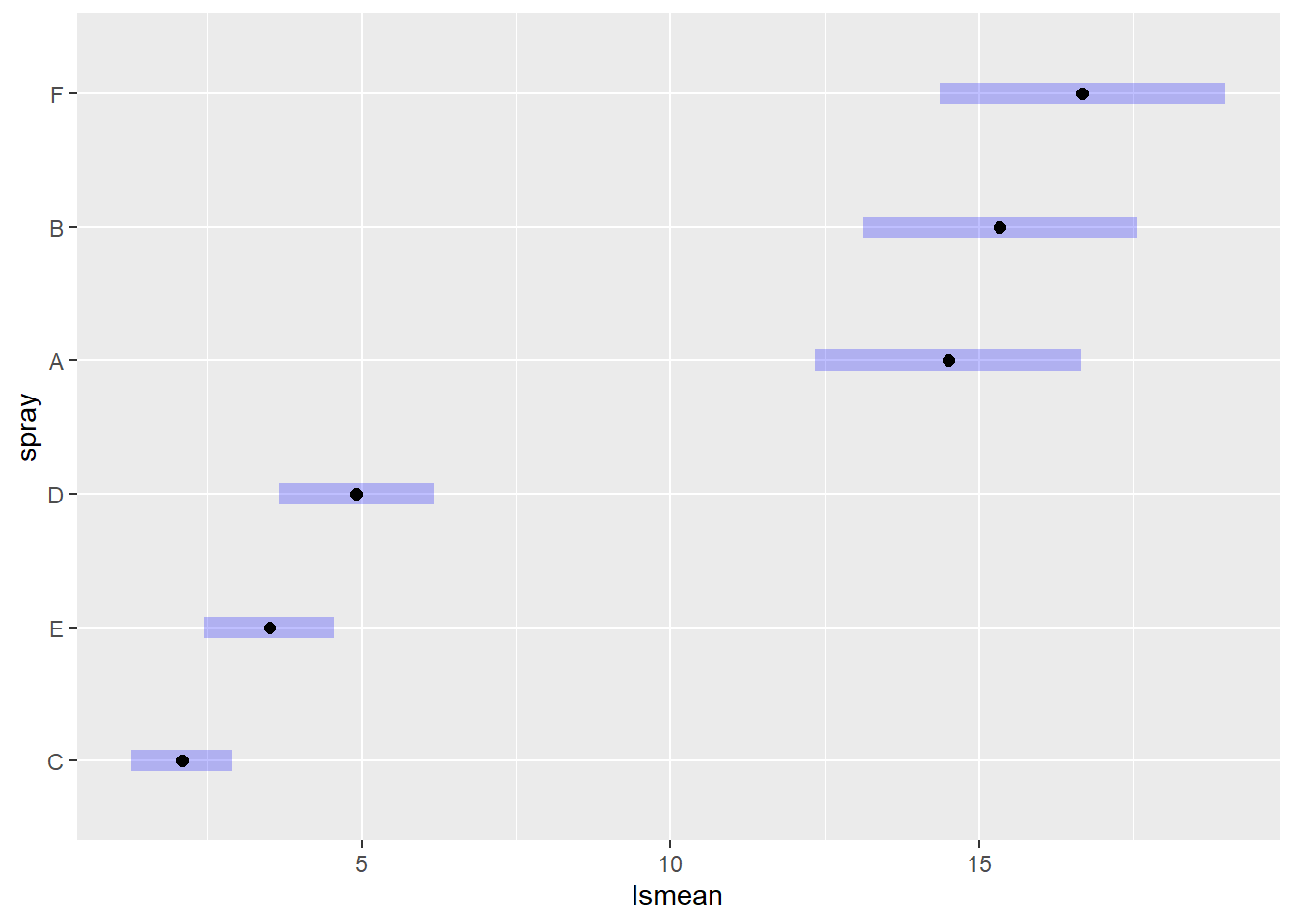
 spray lsmean    SE  df asymp.LCL asymp.UCL .group
 C       2.08 0.417 Inf      1.27      2.90  A    
 E       3.50 0.540 Inf      2.44      4.56  AB   
 D       4.92 0.640 Inf      3.66      6.17   B   
 A      14.50 1.099 Inf     12.35     16.65    C  
 B      15.33 1.130 Inf     13.12     17.55    C  
 F      16.67 1.179 Inf     14.36     18.98    C  

Confidence level used: 0.95 
P value adjustment: tukey method for comparing a family of 6 estimates 
significance level used: alpha = 0.05 
NOTE: If two or more means share the same grouping symbol,
      then we cannot show them to be different.
      But we also did not show them to be the same. 

plot(cld(medias2, by = NULL, Letters = LETTERS, alpha = .05))